Accuracy and Tolerance a short discussion

Accuracy and Tolerance a short discussion

Tolerance and accuracy are two important concepts in engineering that are often related but quite distinct from each other.

Accuracy refers to how close a measured value is to the true or accepted value. It indicates the correctness of a measurement.

Tolerance refers to the permissible limit or limits of variation in a physical dimension or measured value. It defines the range within which a measurement is considered acceptable or compliant with specifications.

In summary accuracy indicates how close a measurement is to the true value whilst tolerance specifies the allowable deviation from a specified value.

Despite the distinction between the two, in the realms of engineering and surveying these concepts begin to get intertwined and somewhat interdependent: Unfortunately what has been determined as achievable survey accuracy using modern measurement technology is often appropriated as a tolerance for engineering, perhaps without due cognizance of a “reasonably achievable” “performance” in the “real world”.

Performance in this case does not refer to the potential for any mistakes or “blunders” in the measurements nor does it allow for so-called systematic, scale or cyclic error. Because all of these sources of error are deemed removable from the performance of the measurement technology through best practice, measurement network design and creation of “redundancy”.

What is left is uncertainty, caused by taking “good” measurements in an imperfect, variable environment. Modelling uncertainty is a big part of the science of applying accuracy to tolerances. This modelling uses knowledge of the Normal Distribution and Probability theory. The distribution and theory describes how random occurrences of variation (uncertainty) group around a “most probable value” which can be quantified in a number of ways but is often termed the average or mean value.

Once a mean or average value is determined its variance can be modelled using its standard deviation – which is calculated by differencing each individual sampled value from the mean and dividing by the number of samples.

Of course for a mean the differences of all samples (some larger, some smaller, in magnitude) would aggregate to zero so in order for this quantity to be meaningful the “sign” of the difference is removed. One way the calculation can then be achieved is by adding the “squares” (value multiplied by itself) of all the differences together, dividing by the sample size and then taking the square root (so as to reverse the process of using the squares).

It is important at this stage in this simplified description to link “factory specifications” for measurement devices to variations in measurements as determined by Normal Distribution methods. Factory specifications are determined by testing and using the same statistical methods to arrive at a stated precision or specification. And this means that the “standard error” for individual measurements can, for all intents and purposes, be treated as the specification = standard deviation = magnitude of variation = precision. Now perhaps it is also understandable as to why “precision” is not the same as “accuracy”. It is how precision is used that determines accuracy.

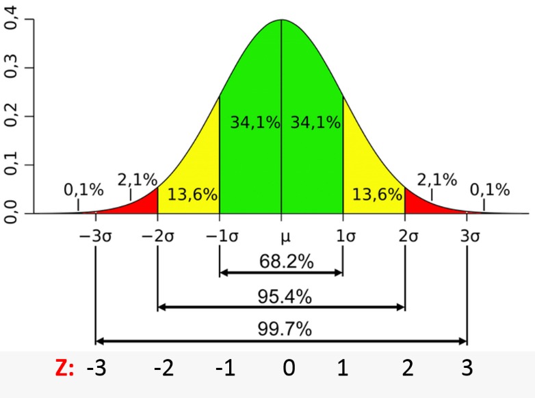
So, in terms of probability the “law” of the Normal Distribution of variance (and remember this is when all other forms of “error” – including blunders - are removed) is that just under 70% of the “outcomes” (the result) will correspond to a value at or below “one standard deviation of the mean”.

Figure 1 Probabilities for standard deviations from the mean in the Normal Distribution.

So in summary the “error” (accuracy) of an individual value should be within one standard deviation of its “population” mean about 70% of the time. However the reality is that another 25% of the time, through no fault of the observer, the error can be twice the size! And then there is a 1 in 300 chance that the error in the value could be as large as three standard deviations from the mean.

It is important to understand that this range of outcomes is for the same “quality” of performance. This is why when you see people jumping up and down and celebrating a near “perfect” outcome it is good to remember that this does not mean that their performance was any better than somebody who achieved a slightly worse result. And this is where understanding the possible outcomes and what may or may not be acceptable becomes really important. For in fact it is the ability to analyze “less than perfect” outcomes and decide on whether anything else could have been reasonably done that is often more important.

Of course, engineering and surveying “results” are mostly made of constituent elements (components) and one way of quantifying uncertainty for a result is to take all the constituent “components” and aggregate the magnitude of their stated uncertainties (standard errors) using the function of the components’ interrelationships with each other.

During this aggregation it is important to recognize that outcomes would include the possibility of all the component uncertainties being in the same “+” or “–“ direction (compounding) plus all the possibilities in-between of some components’ uncertainties being in the opposite direction to others (partly or even completely compensating).

As an example a horizontal co-ordinate position could be a function of a distance and direction from another co-ordinate position. Using the same geometrical rules that created the co-ordinate value the aggregated uncertainty of that co-ordinate can also be calculated. In this case it is evident that the directional error has the potential to magnify its impact on the outcome as a function of the distance over which it is applied.

Nowadays a lot of computation programs for measurement “networks” will now do the work of aggregating the standard errors for the engineer or surveyor and work out the overall uncertainties in the result. Of course, such computations rely upon good estimating of the constituent standard errors.

Overall uncertainties (often stated in surveying as “error ellipses” – which describe the “region” of uncertainty) then really need to be understood in the context of their “probability”. That is, about 70% of the time the overall result will contain between zero and one standard deviation from its average outcome and 99.7% of the time will be within three standard deviations.

The expertise of the engineer and surveyor is really to understand the probabilities and risks associated with this range of outcomes – and certainly with respect to the tolerances they need to satisfy.

With modern day computing it is now possible to design and “pre-analyze” positioning and measurement networks so that the uncertainties at the “delivery points” (where tolerances are applied) are known beforehand. These can then be compared to tolerances to see if the planned approach is fit for purpose.

Please be in touch with MDetail if you have any questions or would like an assessment of your process accuracy and comparison to required tolerances.